US Foreign Policy
Research Methods Primer
2024-09-17
Interpreting and Assessing Statistical Models

Confounding Example
Let’s imagine we’re interested in the relationship between gas pedal pressure and speed, so we collect data on
- A few hundred drivers
- Their speed in mph
- How hard they press the pedal
Call:
lm(formula = speed ~ pedal_pressure, data = cardata)

Coefficients:
   (Intercept)  pedal_pressure
70.0441843 -0.0004776 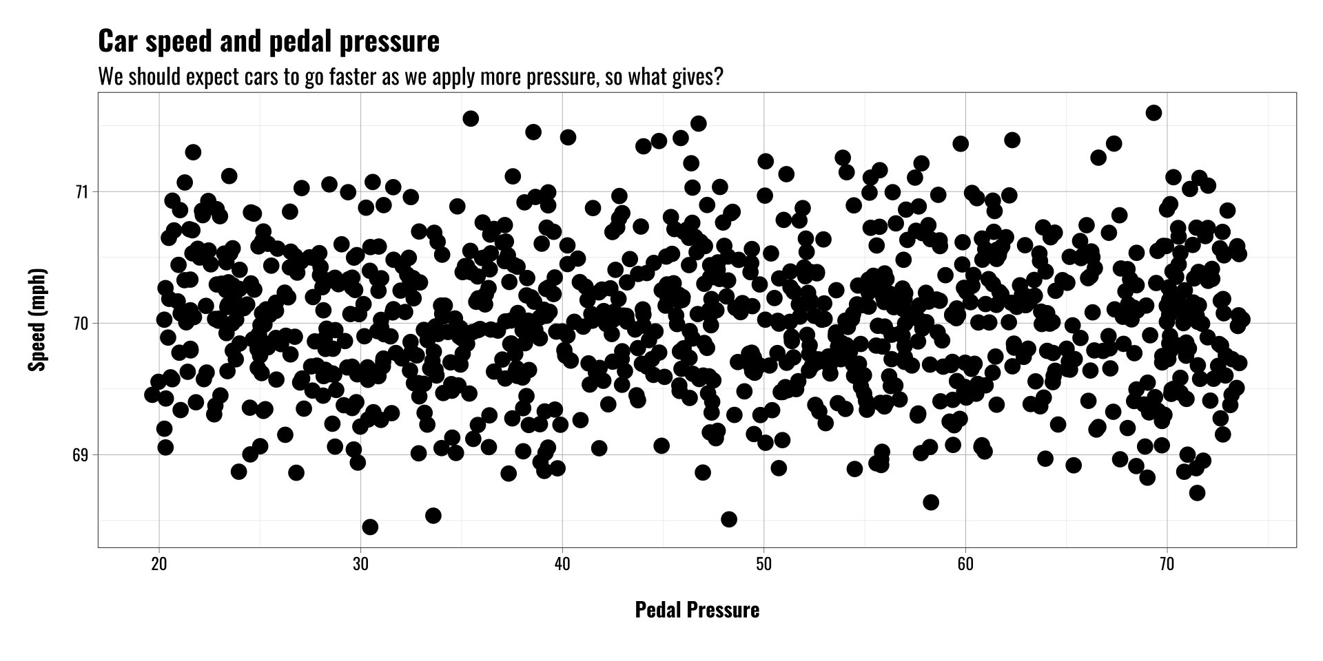
Confounding Example
Confounding can mask causal relationships
We need to understand the data generating process to help us make sense of results that may or may not themselves make sense
Adjusting for confounders in our model can reduce bias and help us better estimate causal relationships
Call:
lm(formula = speed ~ pedal_pressure + incline, data = cardata)

Coefficients:
   (Intercept)  pedal_pressure         incline
45.110 1.244 -1.492 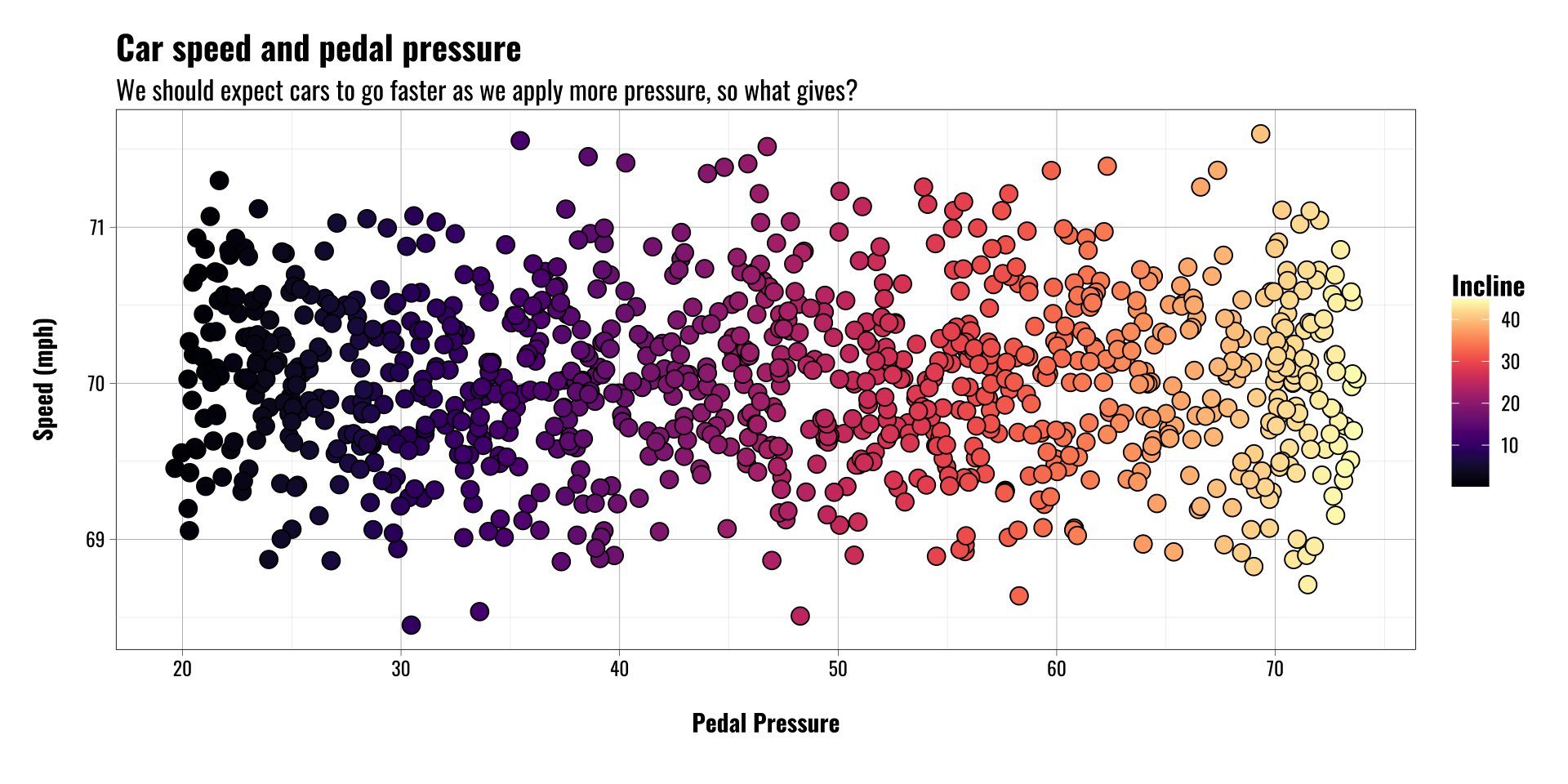
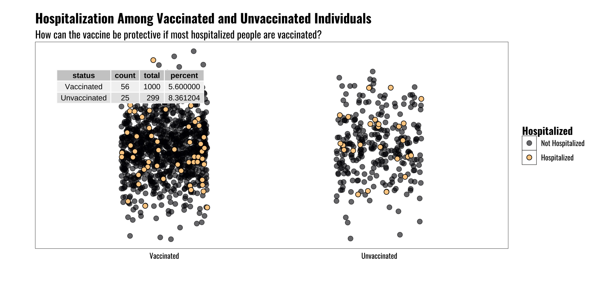
Base Rate Fallacy
What is it and why does it matter?
- Counts can be deceptive without information about population of interest
- Example of vaccine status and hospitalization
- Vaccines are effective at reducing risk of severe illness, hospitalization, etc.
- And yet in some locations we see more hospital beds occupied by vaccinated people than non-vaccinated people
- Huh? What gives?
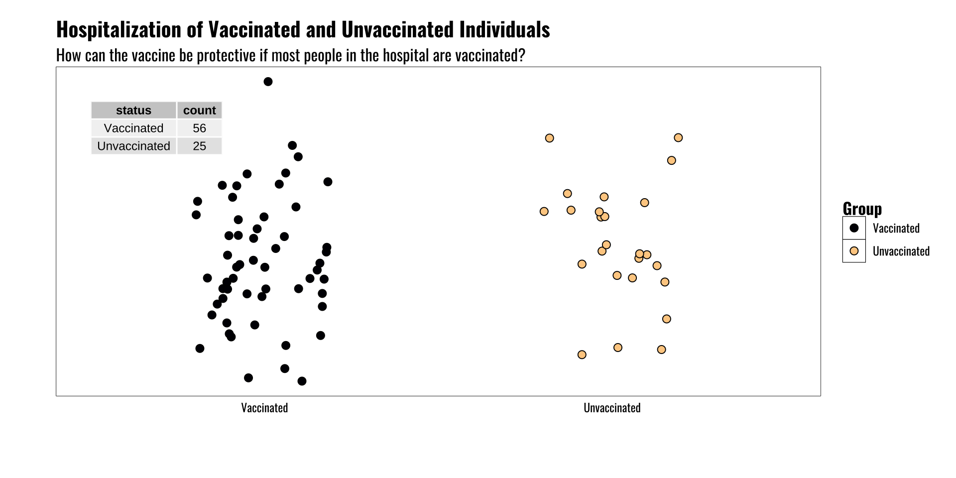
Base Rate Fallacy
The underlying population matters!
The rate of an event may vary across groups
Knowing something about the reference population is key
Another way to think of this is the symmetry/asymmetry of conditional probabilities
\[Pr(H \mid V) \neq Pr(V \mid H)\]
Simpson’s Paradox
Example:
Imagine we have data on the exercise activity and cholesterol of a few hundred adults
We plot the individuals’ cholesterol levels against their level of exercise (we’ll assume we directly observe this and it’s not self-reported)
In the plot we see that exercise appears to correlate positively with cholesterol levels. A simple regression model supports this eyeball estimate.
Call:
lm(formula = y ~ x, data = data2)

Coefficients:
(Intercept)            x
182.372 2.078 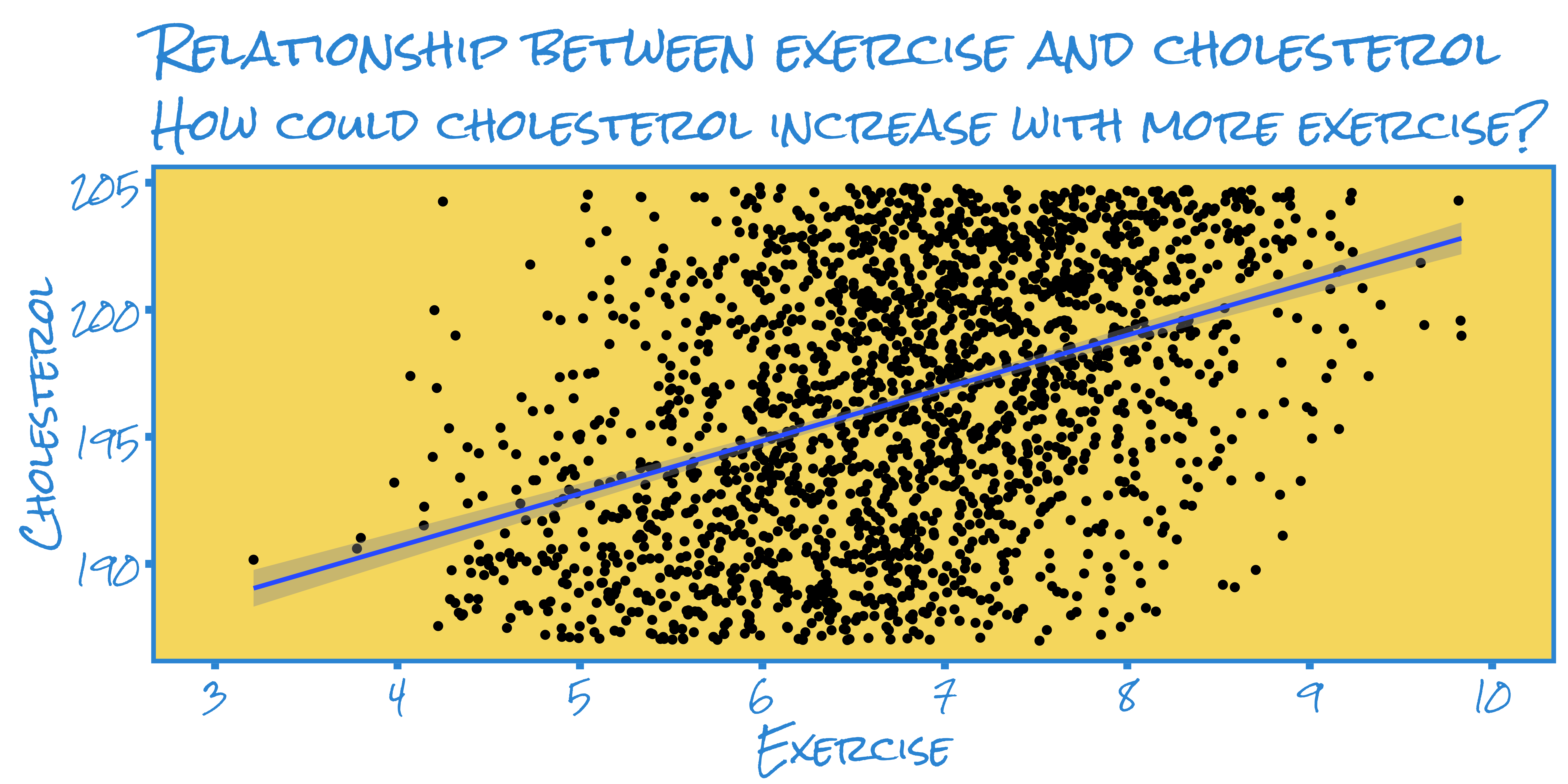
Simpson’s Paradox
Example:
But what if we’re omitting some key variables?
It’s possible for results to reverse if we’re omitting a variable that could also affect cholesterol levels
Another way to say this is that the effect of exercise might be biased because we’re leaving other important things out of the model.
One good variable would be patient age, so let’s see what that looks like
Call:
lm(formula = y ~ x + age, data = data2)

Coefficients:
(Intercept)            x     ageAge 2     ageAge 3     ageAge 4     ageAge 5
193.1930 -0.6774 4.2166 8.1891 11.8306 15.1400 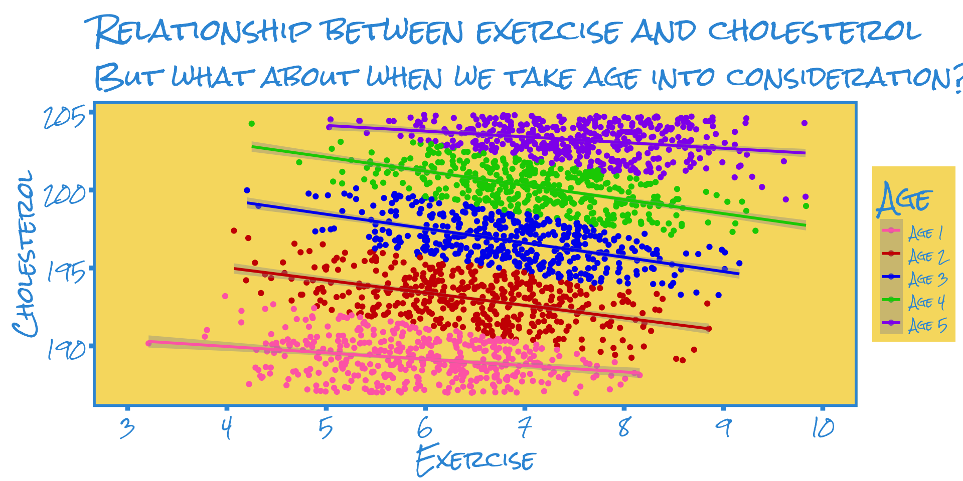
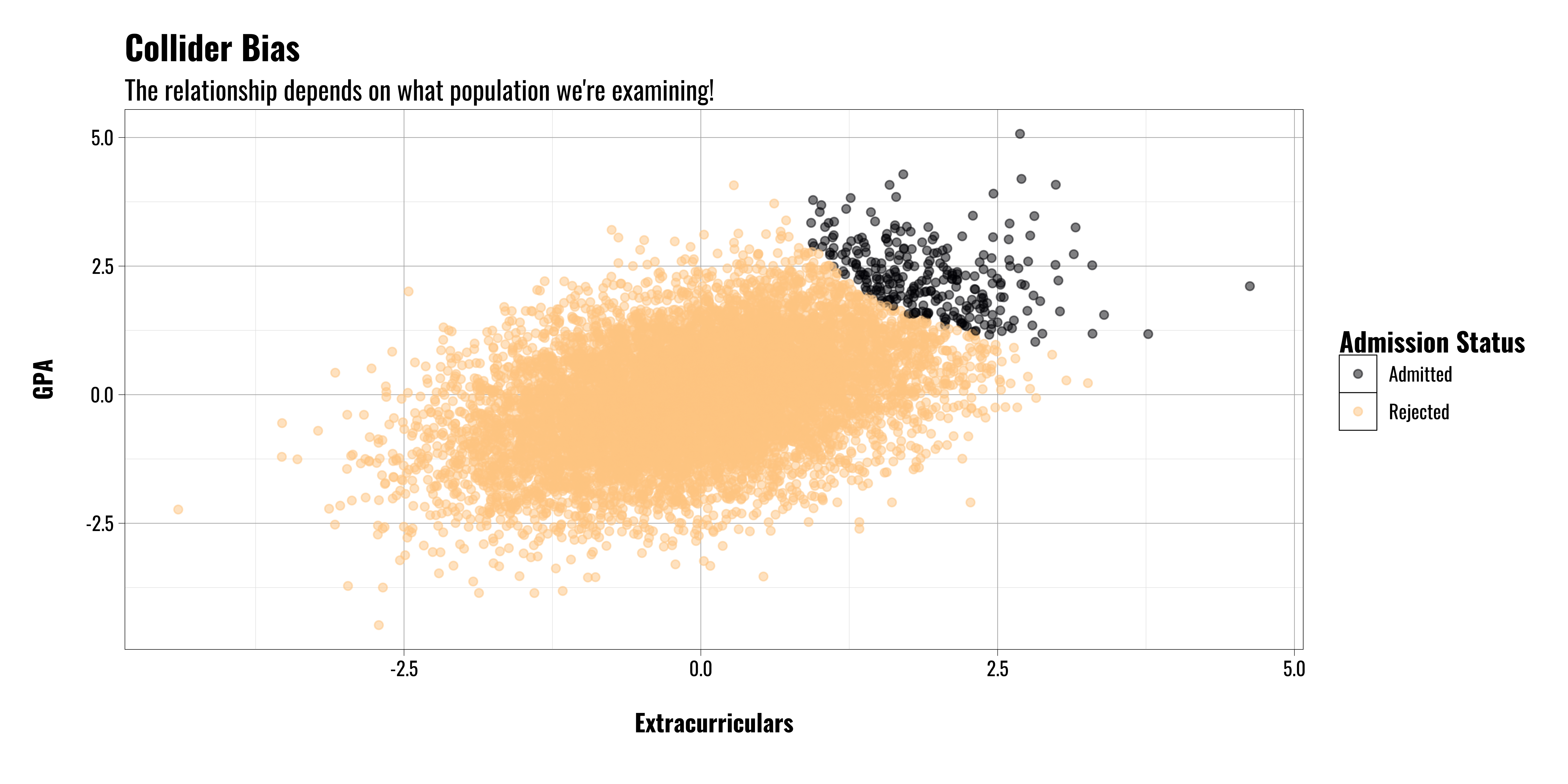
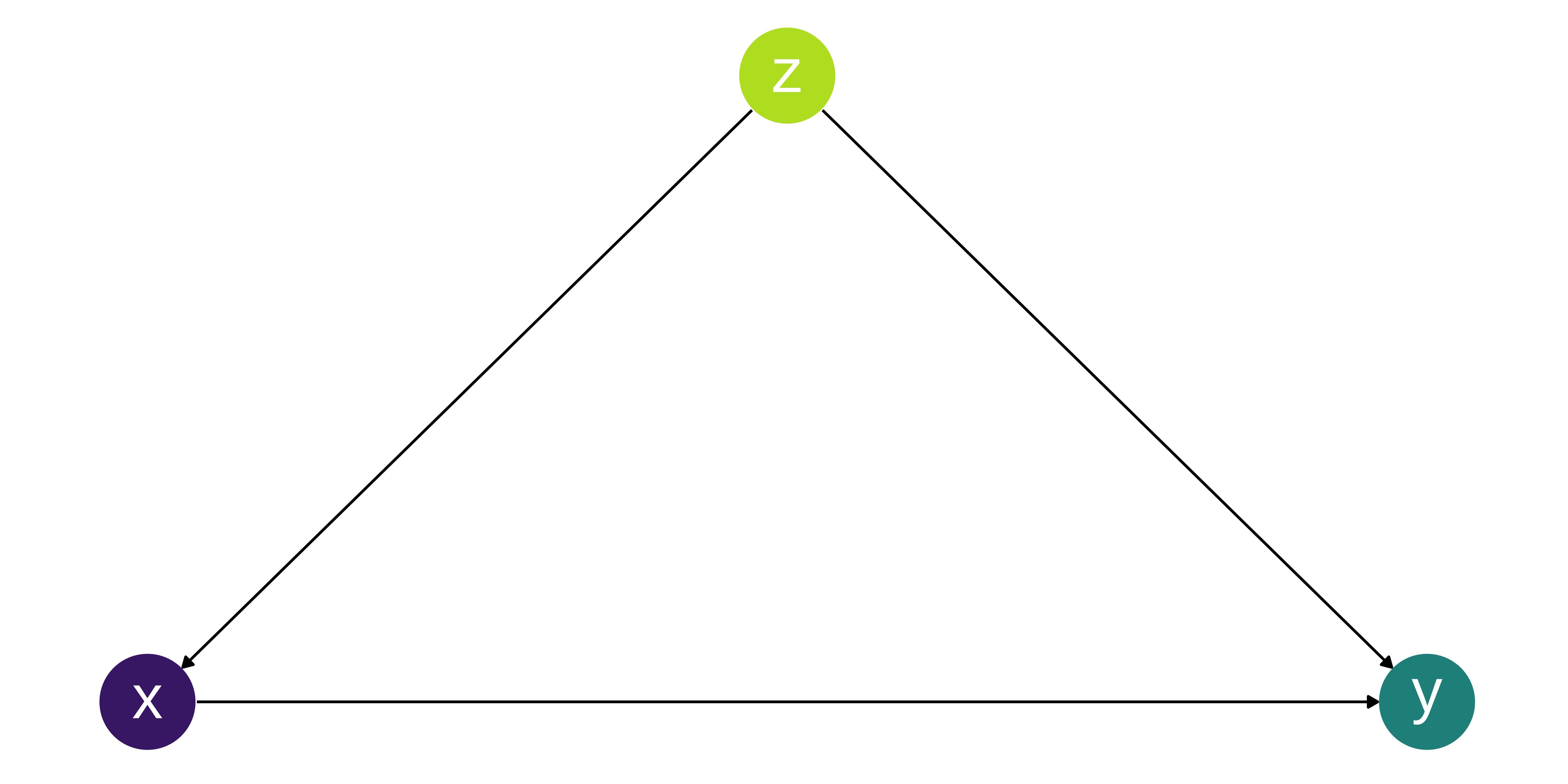
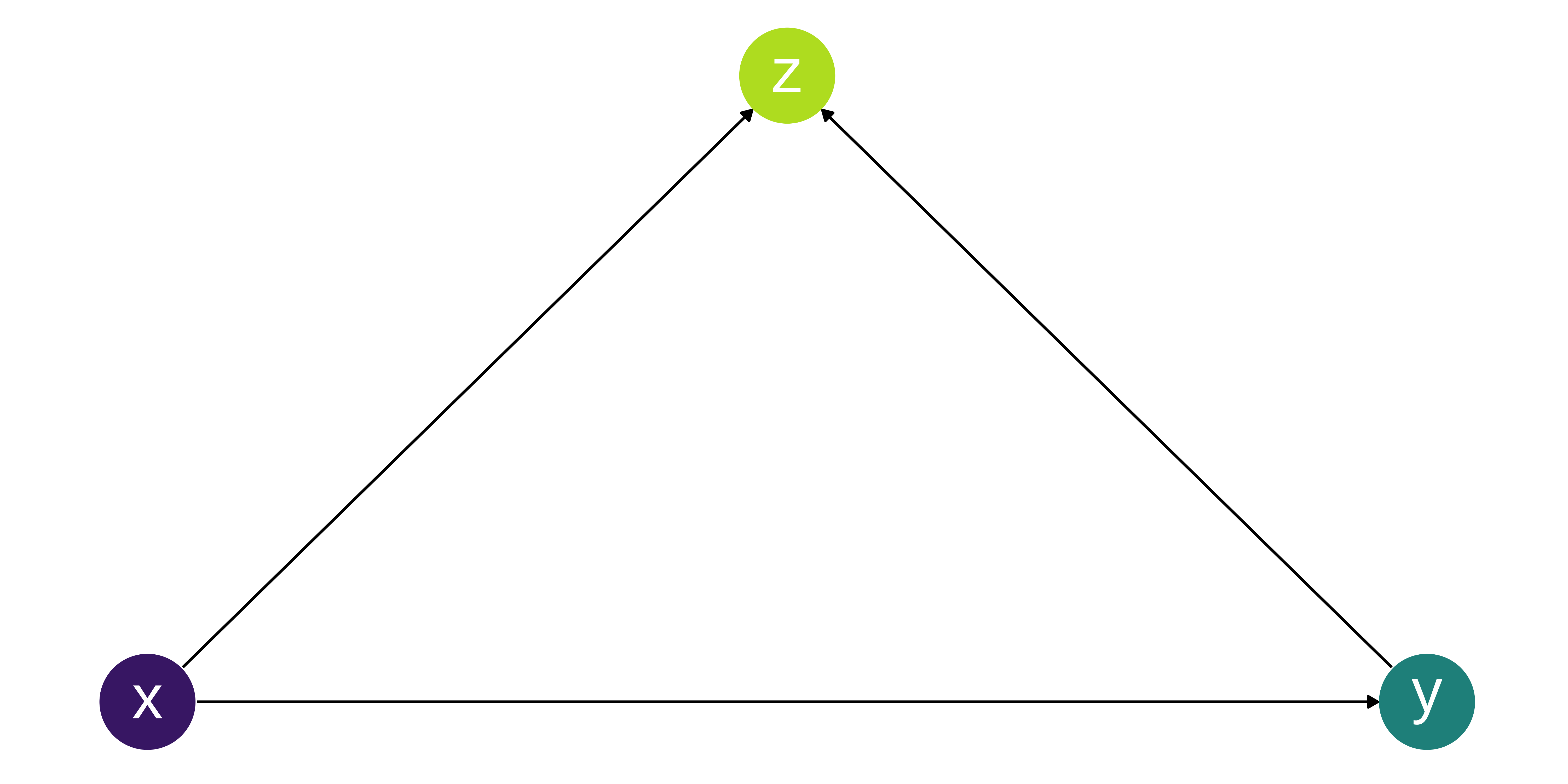
Collider Bias
What is collider bias?
Collider bias can be introduced by adjusting for a common effect.
It can also be a form of selection bias.
Similar to Simpson’s Paradox it can make effects appear to be the opposite of what they are, but also depends on the population of interest.
In this example Z is a collider because both X and Y cause Z.
Collider Bias
Example: College Admissions
Let’s assume we’re interested in looking at students who have been admitted to college to see what the relationship is between their high school extracurricular activities and GPA
We collect data on college freshman and compare their extracurricular activities in high school with their GPA.
Surprisingly, we find a negative relationship.
That’s sad.
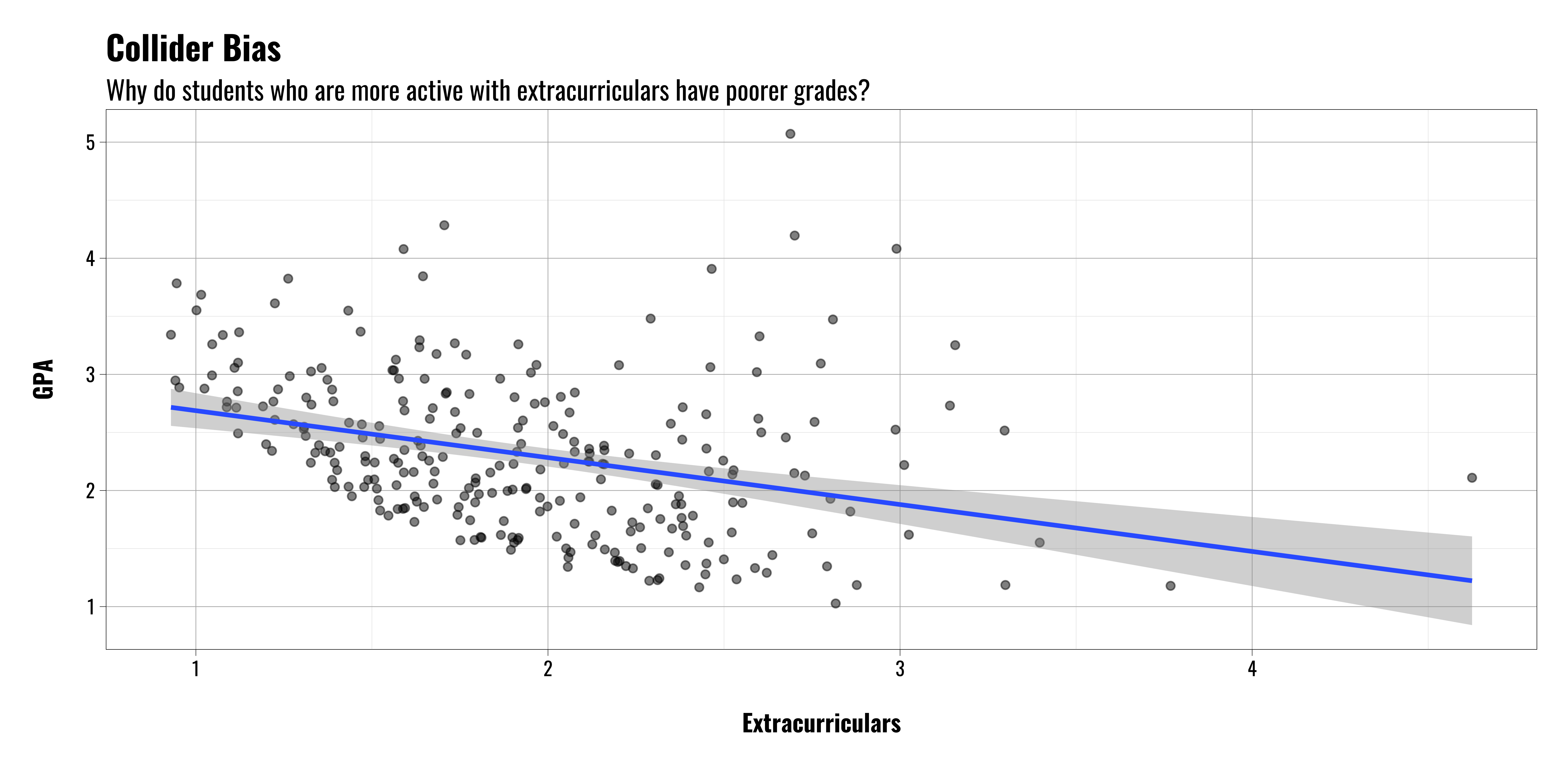
Collider Bias
Example: College Admissions
But wait!
If we’re looking at students who have already been admitted to college we’re implicitly conditioning on a collider variable (i.e. acceptance/admission status)
If we step back and look at the entire population of high school students we find something different
Students who have better grades and/or better extracurricular activities are more likely to be admitted to college in the first place.